by R. Grothmann
based on a notebook by A. Busser
Trefoil knot in almost tubeplot style (the radius is not quite uniform).
>u:=linspace(-pi,pi,160); v:=linspace(-pi,pi,400)'; ...
 x:=(4*(1+.25*sin(3*v))+cos(u))*cos(2*v); ...
 y:=(4*(1+.25*sin(3*v))+cos(u))*sin(2*v); z=sin(u)+2*cos(3*v); ...
 plot3d(x,y,z,frame=0,scale=1.5,hue=1,light=[1,0,-1],zoom=3.2):
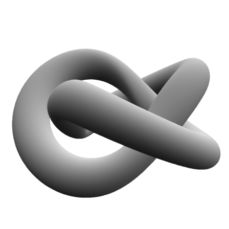
A 3D anaglyph view of this knot.
>plot3d(x,y,z,frame=0,scale=1.5,hue=1,light=[1,0,-1],anaglyph=1,zoom=3.2):
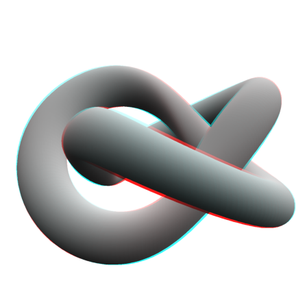
Use red/cyan glasses to view this.
Change the '3's by '5's and you have a 5_1 knot. Surely any torus knot can be obtained this way...
>x:=(4*(1+.4*sin(5*v))+cos(u))*cos(2*v); ...
 y:=(4*(1+.4*sin(5*v))+cos(u))*sin(2*v); z=sin(u)+2*cos(5*v); ...
 plot3d(x,y,z,frame=0,scale=1.5,hue=1,light=[1,0,-1], ...
   zoom=3,anaglyph=1):
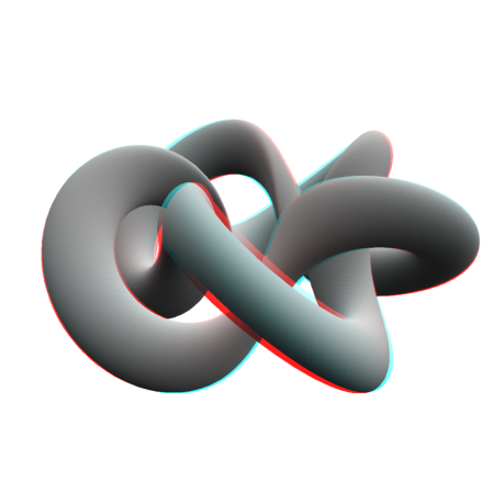
I try to explain this, and improve the look by making the tube more consistent in radius.
First the curve is a based on the curve with the following coordinates.
>function fx (t) &= 4*(1+sin(3*t)/3)*sin(2*t)
                                  sin(3 t)
                      4 sin(2 t) (-------- + 1)
                                     3
>function fy (t) &= 4*(1+sin(3*t)/3)*cos(2*t)
                                  sin(3 t)
                      4 cos(2 t) (-------- + 1)
                                     3
These curves run twice around the unit circle with a periodic alternation in the radius.
>t=linspace(-pi,pi,400); ...
 plot2d(fx(t),fy(t),r=5):
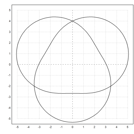
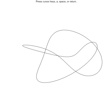
If we add height to this curve, we get a curve forming a 3D knot.
>function fz(t) &= 2*cos(3*t)
2 cos(3 t)
Rotate the figure with the cursor keys to get an impression of the knot. Or press a to generate an anaglyph, if you have red/cyan glasses.
>plot3d(fx(t),fy(t),fz(t),wire=1,>user,zoom=4,<frame, ...
   title=" Press cursor keys, a, space, or return."):
>function f(t) &= [fx(t),fy(t),fz(t)]
                    sin(3 t)                   sin(3 t)
       [4 sin(2 t) (-------- + 1), 4 cos(2 t) (-------- + 1),
                       3                          3
                                                           2 cos(3 t)]
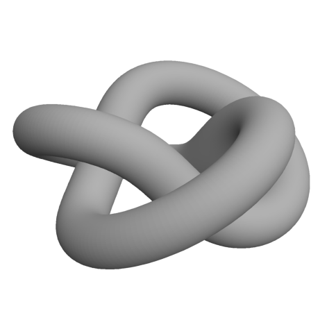
Next we add a tube to the curve.
Instead of a simple rotation of a circle around the x-axis, we compute the derivative vector of the curve.
>function df(t) &= diff(f(t),t)
                    sin(3 t)
       [8 cos(2 t) (-------- + 1) + 4 sin(2 t) cos(3 t),
                       3
                                          sin(3 t)
        4 cos(2 t) cos(3 t) - 8 sin(2 t) (-------- + 1), - 6 sin(3 t)]
                                             3
>function w1(t) &= [df(t)[2],-df(t)[1],0]
                                          sin(3 t)
       [4 cos(2 t) cos(3 t) - 8 sin(2 t) (-------- + 1),
                                             3
                               sin(3 t)
                 - 8 cos(2 t) (-------- + 1) - 4 sin(2 t) cos(3 t), 0]
                                  3
>function w2(t) &= crossproduct(df(t),w1(t));
>function g(s,t,r) &= f(t)+r*(cos(s)*w1(t)/norm(w1(t))+sin(s)*w2(t)/norm(w2(t)));
>function gx(s,t) &= g(s,t,r)[1];
>function gy(s,t) &= g(s,t,r)[2];
>function gz(s,t) &= g(s,t,r)[3];
>s=linspace(pi,-pi,160)';
>r=1;
>fullwindow; plot3d(gx(s,t),gy(s,t),gz(s,t),>hue, ...
    <frame,zoom=5,max=0.7,amb=0):
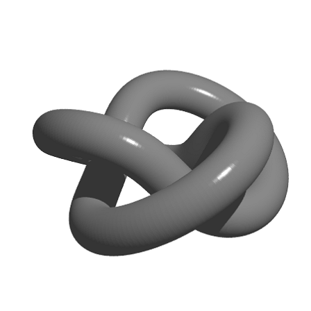
To be able to run this, you need to install Povray and put it into the program path.
>load povray;
>pov3d(gx(s,t),gy(s,t),gz(s,t),zoom=5,axis=0, ...
   look=povlook(gray,>phong));
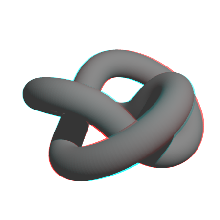
The following scene takes quite a while to write and to parse. Please be patient. On my system, it took about 30 seconds.
>pov3d(gx(s,t),gy(s,t),gz(s,t),zoom=5,axis=0, ...
   look=povlook(gray,),>anaglyph);
Let us clean up, since the Povray source code is quite large.
>povclear();